
ONNX는 Open Neural Network Exchange의 줄인 말로 다른 DNN 프레임워크 환경(ex Tensorflow, PyTorch, etc..)에서 만들어진 모델들을 서로 호환되게 사용할 수 있도록 만들어진 공유 플랫폼입니다.
ONNX를 사용하는 이유는 다음과 같습니다.
- 모델의 호환성을 높일 수 있습니다. 예를 들어, PyTorch로 학습한 모델을 TensorFlow Serving에서 서빙할 수 있습니다.
- 모델의 개발과 유지보수를 쉽게 할 수 있습니다. ONNX는 모델의 구조와 파라미터를 명시적으로 저장하기 때문에, 모델의 개발과 유지보수를 쉽게 할 수 있습니다.
- 모델의 성능을 향상시킬 수 있습니다. ONNX 모델을 TensorFlow Serving에서 실행하면, TensorFlow Serving의 내부 최적화 기법을 사용하여 모델의 성능을 향상시킬 수 있습니다
해당 글은 onnx를 사용하여 MNIST를 구분하는 간단한 모델을 생성하고 서빙까지를 구현한 예제입니다.
전체 코드입니다. colab에서 실행가능하며, CPU만으로도 실습 가능합니다.
1. 패키지 설치 및 정의
pip를 통해 onnx를 설치합니다.
!pip install onnx onnxruntime


import numpy as np
import torch
import torch.nn as nn
import torch.optim as optim
import torchvision
import torchvision.transforms as transforms
import matplotlib.pyplot as plt
2. 데이터 로드
PyTorch를 사용하여 MNIST 데이터셋을 다운로드하고 훈련 세트와 테스트 세트로 나눕니다.
# 예제 데이터 생성 및 DataLoader 설정
transform = transforms.Compose([transforms.ToTensor(), transforms.Normalize((0.5,), (0.5,))])
train_dataset = torchvision.datasets.MNIST(root='./data', train=True, download=True, transform=transform)
train_loader = torch.utils.data.DataLoader(train_dataset, batch_size=64, shuffle=True)
3. 데이터 확인
MNIST 데이터가 어떻게 구성되어있는지는 다음의 코드로 이미지와 라벨을 볼 수 있습니다.
data_iterator = iter(train_loader)
images, labels = next(data_iterator)

# 이미지를 시각화하여 보여주는 함수
def imshow(img):
    # 텐서를 넘파이 배열로 변환
    npimg = img.numpy()
    # 이미지를 (batch_size, height, width)에서 (height, width, batch_size)로 변환
    plt.imshow(np.transpose(npimg, (1, 2, 0)))
    plt.axis('off')  # 축 제거
    plt.show()

# 이미지 시각화
imshow(torchvision.utils.make_grid(images))
print('라벨:', labels)
4. 모델 정의
간단한 신경망 모델을 정의합니다. 간단한 dense 모델을 정의한 신경망입니다.
class SimpleMNISTModel(torch.nn.Module):
    def __init__(self):
        super(SimpleMNISTModel, self).__init__()
        self.flatten = torch.nn.Flatten()
        self.fc1 = torch.nn.Linear(28 * 28, 128)
        self.relu = torch.nn.ReLU()
        self.fc2 = torch.nn.Linear(128, 10)

    def forward(self, x):
        x = self.flatten(x)
        x = self.fc1(x)
        x = self.relu(x)
        x = self.fc2(x)
        return x

# 모델 초기화
model = SimpleMNISTModel()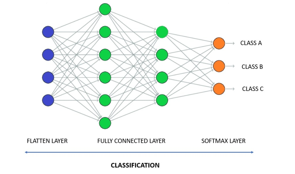
해당 모델의 레이어를 보기 위해 torchsummary패키지를 통해서 레이어를 확인했다.
!pip install torchsummary


from torchsummary import summary
summary(model, (1, 28, 28))


----------------------------------------------------------------
        Layer (type)               Output Shape         Param #
================================================================
           Flatten-1                  [-1, 784]               0
            Linear-2                  [-1, 128]         100,480
              ReLU-3                  [-1, 128]               0
            Linear-4                   [-1, 10]           1,290
================================================================
Total params: 101,770
Trainable params: 101,770
Non-trainable params: 0
----------------------------------------------------------------
1. Flatten-1: 입력 이미지를 1차원으로 평탄화하는 레이어
2. Linear-2: 첫 번째 Fully Connected Layer로, 784의 입력을 받아 128의 출력을 가집니다.
3. ReLU-3: ReLU 활성화 함수
4. Linear-4: 두 번째 Fully Connected Layer로, 128의 입력을 받아 10의 출력을 가집니다.
5. 모델 학습
이제 모델을 학습시킵니다. SGD 알고리즘을 사용하여 손실 함수로 CrossEntropyLoss를 사용합니다.
CrossEntropyLoss는 다중 분류 문제에 사용되는 손실 함수입니다. 이 함수는 모델의 예측 결과와 정답 라벨 사이의 거리를 측정하여 손실값을 계산합니다.
- 다중 분류 문제에 적합
- 확률 분포를 사용하여 손실값을 계산
- 오분류가 발생할수록 손실값이 커짐
학습이 완료되면 모델을 ONNX 형식으로 변환합니다.
# 손실 함수와 옵티마이저 설정
criterion = nn.CrossEntropyLoss()  # 손실 함수
optimizer = optim.SGD(model.parameters(), lr=0.1)  # SGD 옵티마이저


# 학습률(learning rate)과 손실(loss)을 저장할 리스트
learning_rates = []
losses = []

# 모델 학습
epochs = 5
for epoch in range(epochs):
    running_loss = 0.0
    for i, data in enumerate(train_loader, 0):
        inputs, labels = data
        optimizer.zero_grad()
        outputs = model(inputs)
        loss = criterion(outputs, labels)
        loss.backward()
        optimizer.step()
        running_loss += loss.item()
        # 매 100번째 미니배치마다 학습률과 손실을 리스트에 추가
        if i % 100 == 99:
            learning_rates.append(optimizer.param_groups[0]['lr'])
            losses.append(running_loss / 100)
            print(f'Epoch [{epoch + 1}/{epochs}], Step [{i + 1}/{len(train_loader)}], Loss: {running_loss / 100:.4f}')
            running_loss = 0.0

print('학습 완료')

# 모델을 ONNX 형식으로 저장
example_input = torch.randn(1, 1, 28, 28)  # 입력 예제 데이터 생성
torch.onnx.export(model, example_input, "simple_mnist_model.onnx", verbose=True)

print('ONNX 모델 저장 완료')
6. 모델 평가
# 학습률과 손실에 대한 그래프 그리기
plt.figure(figsize=(10, 5))

# 학습률 그래프
plt.subplot(1, 2, 1)
plt.plot(learning_rates, label='Learning Rate', color='blue')
plt.title('Learning Rate per Step')
plt.xlabel('Step')
plt.ylabel('Learning Rate')
plt.legend()

# 손실 그래프
plt.subplot(1, 2, 2)
plt.plot(losses, label='Loss', color='red')
plt.title('Training Loss')
plt.xlabel('Step (per 100 steps)')
plt.ylabel('Loss')
plt.legend()

plt.tight_layout()
plt.show()
7. 서빙
저장된 Onnx 모델을 로드하여, 테스트 데이터로 평가합니다.
import torch
import torchvision
from torchvision import transforms

# MNIST 데이터셋 불러오기
test_dataset = torchvision.datasets.MNIST(root='./data', train=False, download=True, transform=transforms.ToTensor())
test_loader = torch.utils.data.DataLoader(test_dataset, batch_size=1, shuffle=True)

# 저장된 ONNX 모델 불러오기
ort_session = ort.InferenceSession("/content/simple_mnist_model.onnx")
input_name = ort_session.get_inputs()[0].name

# 모델 평가하기
correct = 0
total = 0
with torch.no_grad():
    for images, labels in test_loader:
        output = ort_session.run(None, {input_name: images.numpy()})
        predicted = torch.argmax(torch.tensor(output))
        total += labels.size(0)
        correct += (predicted == labels[0]).sum().item()

accuracy = correct / total
print(f"모델의 정확도: {accuracy * 100:.2f}%")

모델의 정확도: 95.31%
추가적으로 CNN을 활용한 코드도 추가하였습니다. ONNX를 활용한 부분은 크게 달라지지 않습니다.
단순하게 패키지만을 추가하여, 사용하는 함수나 / 기기의 성능을 높힐수 있으므로, 모델 서빙을 할때는 꼭 ONNX를 사용하시기 바랍니다.
참고문서
https://github.com/mattsul/SampleCode/blob/main/MatthewSullivan_CSE446_HW4_A4.py
https://tutorials.pytorch.kr/advanced/super_resolution_with_onnxruntime.html
'ML > MLops' 카테고리의 다른 글
| [system design] 유해 콘텐츠 감지 (1) | 2024.03.16 |
|---|---|
| onnx model Quantization (0) | 2024.03.11 |
| 파이프라인 구축 (with NES / notebook exceute system) (0) | 2024.01.01 |
| 3. 각 회사별 MLops (0) | 2023.12.25 |
| 2. MLops 아키텍처 (1) | 2023.12.23 |


